Why Minimize Negative Log Likelihood?
One of the wonders of machine learning is the diversity of divergent traditions from which it originates, from classical statistics (both frequentist and Bayesian) to information and control theories, plus a significant dose of pragmatism from computer science. For those interested in the historical relationship between statistics and machine learning, see Breiman’s Two Cultures.
This diversity is reflected in the surprising complexity in answering simple-sounding questions, which often speaks to the heart of trading using computational machine learning models—ranging from estimating HMM models via MLE (e.g. vol / correlation regime models) to non-convex optimization via non-standard likelihood or loss functions (e.g. portfolio optimization via omega):
Why is minimizing the negative log likelihood equivalent to maximum likelihood estimation (MLE)?
Or, equivalently, in Bayesian-speak:
Why is minimizing the negative log likelihood equivalent to maximum a posteriori probability (MAP), given a uniform prior?
Answering this question provides insight into the foundations of machine learning, as well as connection with several branches of mathematics.
Classic statistics opens the answer, beginning with the definition of a likelihood function:

Applying the natural log function in this context is handy, for several reasons. First, numerical analysis reminds us that logs reduce potential for underflow, due to very small likelihoods. Second, calculus reminds us logs permit the addition trick: converting a product of factors into a summation of factors (as seen before in Why Log Returns?). Finally, calculus again reminds us that the natural log function is a monotone transformation.
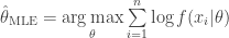
Thus, the extrema of 


From which the maximum likelihood estimator 
As an aside, Bayesians will remind us we can generalized into a MAP estimator, given uniform prior 

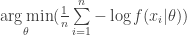
From which optimization and real analysis reminds us of the following equivalence, for all 
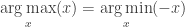
Thus, the following are equivalent:

From this, we technically have an answer to the above two questions on equivalence. Yet, from here lies the opportunity to continue and uncover the relationship between MLE/MAP and both entropy and loss via Kullback-Leibler divergence (KL). To get there, consider the statistical average of the above:
Which converges, by the strong law of large numbers, to the expectation:
![E[- \log f(x|\theta)]](https://s0.wp.com/latex.php?latex=E%5B-+%5Clog+f%28x%7C%5Ctheta%29%5D+&bg=ffffff&fg=333333&s=0&c=20201002)
Which is interesting when considering the difference in distribution between 

![E[\log f(x|\theta^*) - \log f(x|\theta)] = E[\log\frac{f(x|\theta^*)}{f(x|\theta)}] = \int \log \frac{f(x|\theta^*)}{f(x|\theta)} f(x|\theta^*) dx](https://s0.wp.com/latex.php?latex=E%5B%5Clog+f%28x%7C%5Ctheta%5E%2A%29+-+%5Clog+f%28x%7C%5Ctheta%29%5D+%3D+E%5B%5Clog%5Cfrac%7Bf%28x%7C%5Ctheta%5E%2A%29%7D%7Bf%28x%7C%5Ctheta%29%7D%5D+%3D+%5Cint+%5Clog+%5Cfrac%7Bf%28x%7C%5Ctheta%5E%2A%29%7D%7Bf%28x%7C%5Ctheta%29%7D+f%28x%7C%5Ctheta%5E%2A%29+dx+&bg=ffffff&fg=333333&s=0&c=20201002)
Which is indeed equal to none other than the KL divergence, 


Which information theory reminds us is relative entropy, and thus is also equal to the excess risk for the loss function defined by the negative log-likelihood. Finally, connecting Bayesian statistics to the foundation of information theory: gain in Shannon entropy going from prior to posterior is indeed the KL divergence.
Thus, maximum likelihood and maximum a posteriori probability are special case loss functions (see Loss Function Semantics for more on loss semantics in ML).

Nice writeup!
I wonder, why you define the (log-) likelihood function in terms of a full factorization of x. To me that seems to be the mean-field approximation of f(x|theta) as in variational Bayes. Shouldn’t the general case be \prod( x_i | \theta, x_{i+1},…,x_n) to keep the dependencies between the xi?
Nice post. Two more interesting questions though are the following: 1) why MLE “works”? In what sense does it work? 2) Why Bayes MAP works, and in what regime is it close to MLE.
@gappy: good to hear from you; thanks for complement. Agree those are very interesting questions, especially in the pragmatic ML sense of “work”, meaning the estimated parameters generate effective out-of-sample prediction (which, arguably, is what really matters for trading).
Nice writeup.
Though I use MLE a lot, explicitly or implicitly (where for example LSQ is a MLE estimator on series with normal errors), I find MLE to be problematic in the financial space because more often than not we do not know the distribution OR one can take a snapshots of the empirical distribution for some lookback period, but do not know how it evolves.
Of course there are approaches that attempt to determine the distribution and its evolution, such as particle filters or other forms of sampling. These encounter problems with outliers and sparse data though.
ML techniques become more valuable, particularly in situations where the distribution is not known and/or dimensionality is high.
@tr8dr: thanks; good to hear from you, given your blog has been quiet for a while. Agree with your comments. To gappy’s question above and your comment about ML value, curious what you think of Bayesian methods vis-a-vis distribution uncertainty: given strong uncertainty on distribution, do you prefer MLE methods or applying Bayesian methods and hoping robustness guides increasingly accurate posterior iteration?
Reblogged this on Convoluted Volatility – StatArb,VolArb; Macro..
This is kind of overlooking the real point: asymptotic consistency (maximum likelihood will recover the true distribution given enough samples) and asymptotic efficiency (it gets close to the true distribution pretty fast as you add samples).