Minimum Variance Portfolios
As recounted in Portfolio Theory is Dead, Now What?, the minimum variance portfolio is the optimal portfolio in a world with zero risk premium. This post expands on the topic via practical implementation in R, preceded by walk through of the corresponding mathematics.
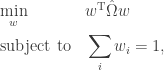
Recall the classic Markowitz mean-variance optimal portfolio is the solution to:

where 


From this starting point, consider two assumptions which lead to the minimum variance portfolio:
- Risk premium is zero
- Aversion to risk is infinite, thus

With those assumptions, the above optimization reduces to the following covariance minimization:
For portfolios constructed from individual stocks (as opposed to sectors, for example), an upper bound 

Jagannathan and Ma (2002) show this constraint improves estimation by amplifying shrinkage efficacy. The authors demonstrate a similar statistical shrinkage benefit provided by the zero lower bound.
Although this is a rudimentary constrained optimization problem, what makes it fun is the “Markowitz optimization enigma”: robustly estimating the covariance matrix 
- Asymptotic Components with Hetersokedastic Factor Residuals
Following Falkenstein, use Connor and Korajczyk (1993) and Jones (2001) to estimate


Where 


- Bayesian Sample Shrinkage Estimator
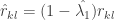
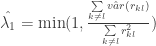
Similar to Nogales, use Ledoit and Wolf (2004) to estimate
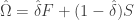


where 


- Sample Variance and Correlation Shrinkage Estimator
Following Schäfer and Strimmer (2005) and Opgen-Rhein and Strimmer (2007) to estimate


Now consider the R necessary to generate these portfolios. Readers seeking more background on portfolio optimization in R are referred to R Tools for Portfolio Optimization by Yollin (R/Finance 2009).
The most important detail is choice of covariance estimator, including Schäfer-Strimmer-Opgen-Rhein from corpcor package and Ledoit-Wolf from tawny package (both functions confusingly named cov.shrink). The Ledoit-Wolf estimator will be used in this and subsequent posts.
These optimizations can be formulated as quadratic programming, and solved using solve.QP from quadprog, via formulating the above optimizations into the following functional form (following Goldfarb and Idnani (1982, 1983)) with a zero 

Assume X is a matrix of log returns, then generate optimization inputs:
<code>covar <- cov.shrink(X)
N <- ncol(X)
zeros <- array(0, dim = c(N,1))
Evaluate the optimization to generate minimum variance portfolio without short selling constraint:
aMat  <- t(array(1, dim = c(1,N)))
res <- solve.QP(covar, zeros, aMat, bvec=1, meq = 1)
Or, similar optimization with short selling constraint (i.e. non-negative weights):
aMat <- cbind(t(array(1, dim = c(1,N))), diag(N))
b0 <- as.matrix(c(1, rep.int(0,N)))
res <- solve.QP(covar, zeros, aMat, bvec=b0, meq = 1)
Finally, return portfolio attributes (similar to portfolio.optim):
y <- X %*% res$solution
port <- list(pw = round(res$solution,3), px = y, pm = mean(y), ps = sd(y))
One minor numerical analysis reminder: use of solve.QP with short selling constraints may generate weights with a negative sign (e.g. -3.417223e-17), due to floating point precision and numerical stability. Such weights are equal to zero when rounded to a reasonable number of digits.
A subsequent post will apply these minimum variance optimization to building and evaluating risk for rotation strategies.
Trackbacks
- FT Alphaville » Further reading
- Minimum Variance Sector Rotation « Quantivity
- Combo: Minima Varianza + R « Quantitative Finance Club
- Minimum Variance Sectors: Part 2 « Quantivity
- Global Rotation with Minimum Variance « Quantivity
- Higher Moments and Minimum Variance « Quantivity
- Empirical Distributions: Minimum Variance « Quantivity
- Momentum: Review « Quantivity
- Momentum Redux « Quantivity
- Markowitz Problem in R | Aaron Crowley
- Portfolio Optimization | Trading and travelling and other things
- Why does the minimum variance portfolio provide good returns? | CL-UAT
- Why does the minimum variance portfolio provide good returns? - Finance Money

Hi,
I tried the same procedure to get a minimum variance portfolio, but I am getting large weights for 1 or 2 individual stocks.
Is there a way to run solveQP with the constraint that the absolute value of the weights are less than some positive number?
Thanks…
@agathocles: no, an epsilon constraint makes the problem not suitable for
solve.QP. If you are interested, I can write a follow-up post that walks through adding such constraints and corresponding R.Btw: I concur with your intuition to avoid portfolios composed of individual equities with large weights (as opposed to sectors or countries, for example), due to idiosyncratic risk.
I would be interested in the follow up post of the problem mentioned above.i.e how to optimise a portfolio in R, with constraints on the weights of the individual assets held in the portfolio and the constraint of the sum of the weights in the portfolio summing to 1.
I have tried to do this using the optim function in R, setting the minimum & maximum tolerances as lower and upper bounds but once I set the constraint of the weights summing to 1 in the function, it creates an error.
I’ve just started playing about with modifications to the optimal mean-variance portfolio in Excel (an initial spreadsheet is here http://optimizeyourportfolio.blogspot.com/2011/05/markowitz-portfolio-optimization.html). This is a good summary of the theory, and motivates me to try R.
Hi, nice post and blog! I’m sorry to comment on this now but would you mind posting the R code for the constrained optimization problem for your 130/30 strategy in the same way that you did in this post? it would be great. Many thanks in any case.
Very nice straightforward coding!
For the questioners looking to apply constraints, check out rMetrics (fPortfolio package) which supports all sorts of adaptation of MVO approaches.
How would you add a transaction cost constraint when rebalancing ?
Thank you for the post. Can you please clarify some of the variable that are not mentioned already? It may be easy to find them in the relevant reference, but it may make it easy to follow here too. For example, what is pi^hat? phi^hat? lambda_1, and 2? etc. Thank you.