Index Return Decomposition

Unmasking a phenomenon into its constituent parts , via functional decomposition , is one of the great beauties of mathematics:

   

This technique finds surprisingly often use in quant models.

Ongoing analysis and trading based on proxy hedging, exemplified by series beginning with Proxy / Cross Hedging, suggests potential for an equity decomposition model based on the relationship between returns of a stock and its corresponding index :

   

To explain this model, let’s build it up from intuition.

To begin, consider a trading observation: interday returns of individual stocks have a subtle relationship with their corresponding index. On some days, return for a given stock follows its index; other days, returns of stock and index diverge strongly. This distinction in behavior is commonly attributed to stock-specific “news”, interpreted broadly—whether known publicly or only privately.

This intuition can be formalized into two-state regime:

• Uninformed regime: stock return follows an index , scaled by a proportional factor
• Informed regime: stock return follows an idiosyncratic path , conditionally independent of its index

Relationship between regimes can be modeled in two ways via . A switching model arises when regimes are binary: . An ensemble model arises when regimes are smooth: . For the latter, can be understood as proportional decomposition weighting of the respective return series, and thus can provide smooth mixing between the regimes. Finally, sign of returns are explicitly decomposed as , acknowledging greater regularity of absolute-valued return series.

Worth noting is the following are latent variables: idiosyncratic path from the informed regime, proportional factor , and regime parameter . Obviously, challenge of this model lies in their estimation. One potential trick is to exploit triangular relationships, as described below.

One stylized fact not explicitly accommodated by this model is well-known asymmetry of uninformed regimes, arising from analysis of market breadth: stocks uniformly go down together (think big down days), but much less often uniformly go up together (majority of rallies). Unclear whether this fact naturally arises via or needs to be explicitly modeled.

Readers familiar with machine learning (ML) may recognize how to reformulate this as an additive model:

   

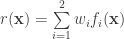
Where .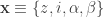

This model can be interpreted in numerous ML ways, depending on the desired objective. For example, and can be interpreted as basis functions. Alternatively, boosting can be applied by interpreting them as weak classifiers. Graphical models can be applied by introducing conditional dependence between , , and . Hierarchical models and decision trees naturally arise when and are further functionally decomposed.

Given this model, an interesting question is how to use it predicatively—whether directional or not. For example, combining models for two stocks which share a common index to introduce the notion of equity triangle arbitrage on the joint .